How to Find Population Mean From Sample Using Bayesian Methods
Bayesian Analysis of a Population Mean (Known SD)
In this chapter we'll consider Bayesian Analysis for the population mean of a numerical variable. Throughout we'll assume that the population standard deviation is known. This is an unrealistic assumption that we'll revisit later.
Example 11.1 Recall Example 4.5 and Example 4.6. Assume body temperatures (degrees Fahrenheit) of healthy adults follow a Normal distribution with unknown mean \(\theta\) and known standard deviation \(\sigma=1\). Suppose we wish to estimate \(\theta\), the population mean healthy human body temperature. Previously we considered a discrete prior distribution for \(\theta\), and grid approximation. Now we'll assume a continuous prior distribution for \(\theta\). Namely, assume the prior distribution of \(\theta\) is a Normal distribution with mean 98.6 and standard deviation 0.7.
- Write an expression for the prior distribution of \(\theta\).
- Suppose a single temperature value of 97.9 is observed. Write the likelihood function.
- Write an expression for the posterior distribution of \(\theta\) given a single temperature value of 97.9.
- Now consider the original prior again. Determine the likelihood of observing temperatures of 97.9 and 97.5 in a sample of size 2, and the posterior distribution of \(\theta\) given this sample. Make a plot of the prior, the scaled likelihood, and the posterior.
- Consider the original prior again. Suppose that we take a random sample of two temperature measurements, but instead of observing the two individual values, we only observe that the sample mean is 97.7. Determine the likelihood of observing a sample mean of 97.7 in a sample of size 2, and the posterior distribution of \(\theta\) given this sample. Make a plot of the prior, the scaled likelihood, and the posterior. Compare to the previous part; what do you notice? (Hint: if \(\bar{Y}\) is the sample mean of \(n\) values from a \(N(\theta, \sigma)\) distribution, what is the distribution of \(\bar{Y}\)?)
Solution. to Example 11.1
-
Remember that in the prior distribution \(\theta\) is treated as the variable. \[ \pi(\theta) \propto \exp\left(-\frac{1}{2}\left(\frac{\theta - 98.6}{0.7}\right)^2\right) \]
-
The likelihood is the Normal(\(\theta\), 1) density evaluated at 97.9, viewed as a function of \(\theta\). \[ f(97.9|\theta) \propto \exp\left(-\frac{1}{2}\left(\frac{97.9-\theta}{1}\right)^2\right) \]
-
Posterior is proportional to likelihood times prior \[ \pi(\theta|y = 97.9) \propto \exp\left(-\frac{1}{2}\left(\frac{\theta - 98.6}{0.7}\right)^2\right)\exp\left(-\frac{1}{2}\left(\frac{97.9-\theta}{1}\right)^2\right) \] After some algebra, you can show that as a function of \(\theta\) this expression represents a Normal distribution.
-
Assuming a random sample, the two temperature measurements are independent. So the likelihood of the pair (97.9, 97.5) is the product of the likelihood of each value. Again, the posterior is proportional to likelihood times prior. \[ {\scriptstyle \pi(\theta|y = (97.9, 97.5)) \propto \exp\left(-\frac{1}{2}\left(\frac{\theta - 98.6}{0.7}\right)^2\right)\left[\exp\left(-\frac{1}{2}\left(\frac{97.9-\theta}{1}\right)^2\right)\exp\left(-\frac{1}{2}\left(\frac{97.5-\theta}{1}\right)^2\right)\right] } \] After some algebra, you can show that as a function of \(\theta\) this expression represents a Normal distribution.
theta = seq(95, 101, 0.0001) # the grid is just for plotting # prior prior = dnorm(theta, 98.6, 0.7) # likelihood likelihood = dnorm(97.9, theta, 1) * dnorm(97.5, theta, 1) # posterior posterior = prior * likelihood posterior = posterior / sum(posterior) / 0.0001 # density scale # plot ymax = max(c(prior, posterior)) scaled_likelihood = likelihood * ymax / max(likelihood) plot(theta, prior, type= 'l', col= 'orange', xlim= range(theta), ylim= c(0, ymax), ylab= '', yaxt= 'n') par(new=T) plot(theta, scaled_likelihood, type= 'l', col= 'skyblue', xlim= range(theta), ylim= c(0, ymax), ylab= '', yaxt= 'n') par(new=T) plot(theta, posterior, type= 'l', col= 'seagreen', xlim= range(theta), ylim= c(0, ymax), ylab= '', yaxt= 'n') legend("topleft", c("prior", "scaled likelihood", "posterior"), lty= 1, col= c("orange", "skyblue", "seagreen"))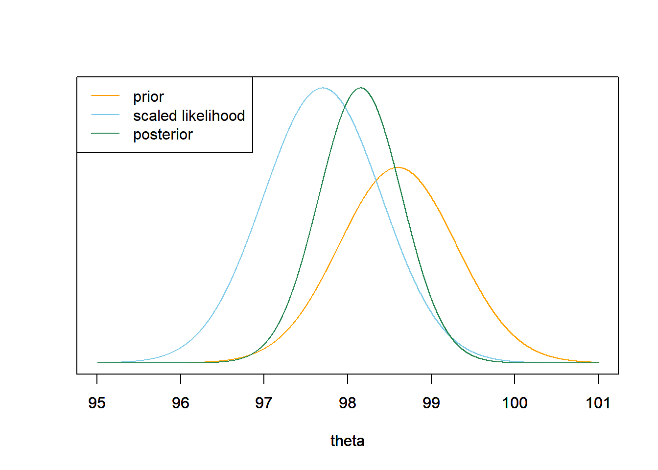
-
If \(\bar{Y}\) is the sample mean of \(n\) values from a \(N(\theta, \sigma)\) distribution, then \(\bar{Y}\) follows a \(N(\theta, \sigma/\sqrt{n})\) distribution. To evaluate the likelihood of a sample mean of 97.7, evaluate the Normal(\(\theta\), \(1/\sqrt{2}\)) density at 97.7, viewed as a function of \(\theta\). Again, the posterior is proportional to likelihood times prior \[ \pi(\theta|\bar{y} = 97.7) \propto \exp\left(-\frac{1}{2}\left(\frac{\theta - 98.6}{0.7}\right)^2\right)\exp\left(-\frac{1}{2}\left(\frac{97.7-\theta}{1/\sqrt{2}}\right)^2\right) \] We see that the posterior distribution is the same as in the previous part.
theta = seq(95, 101, 0.0001) # the grid is just for plotting # prior prior = dnorm(theta, 98.6, 0.7) # likelihood likelihood = dnorm(97.7, theta, 1 / sqrt(2)) # posterior posterior = prior * likelihood posterior = posterior / sum(posterior) / 0.0001 # density scale # plot ymax = max(c(prior, posterior)) scaled_likelihood = likelihood * ymax / max(likelihood) plot(theta, prior, type= 'l', col= 'orange', xlim= range(theta), ylim= c(0, ymax), ylab= '', yaxt= 'n') par(new=T) plot(theta, scaled_likelihood, type= 'l', col= 'skyblue', xlim= range(theta), ylim= c(0, ymax), ylab= '', yaxt= 'n') par(new=T) plot(theta, posterior, type= 'l', col= 'seagreen', xlim= range(theta), ylim= c(0, ymax), ylab= '', yaxt= 'n') legend("topleft", c("prior", "scaled likelihood", "posterior"), lty= 1, col= c("orange", "skyblue", "seagreen"))
It is often not necessary to know all the individual data values to evaluate the shape of the likelihood as a function of the parameter \(\theta\), but rather simply the values of a few summary statistics.
For example, when estimating the population mean of a Normal distribution with known standard deviation \(\sigma\), it is sufficient to know the sample mean for the purposes of evaluating the shape of the likelihood of the observed data under different potential values of the population mean.
In the previous example we saw that if the values of the measured variable follow a Normal distribution with mean \(\theta\) (and known SD) and the prior for \(\theta\) follows a Normal distribution, then the posterior distribution for \(\theta\) given the data also follows a Normal distribution. Performing some algebra on the product of the Normal prior and the Normal likelihood, we can show the following.
Normal-Normal model. Consider a measured variable \(Y\) which, given \(\theta\), follows a Normal\((\theta, \sigma)\) distribution, with \(\sigma\) known. Let \(\bar{y}\) be the sample mean for a random sample of size \(n\). Suppose \(\theta\) has a Normal\((\mu_0, \tau_0)\) prior distribution. Then the posterior distribution of \(\theta\) given \(\bar{y}\) is the Normal\((\mu_n, \tau_n)\) distribution, where
\[\begin{align*} \text{posterior precision:} & &\frac{1}{\tau_n^2} & = \frac{1}{\tau_0^2} + \frac{n}{\sigma^2}\\ \text{posterior mean:} & & \mu_n & = \left(\frac{\frac{1}{\tau_0^2} }{\frac{1}{\tau_0^2} + \frac{n}{\sigma^2}}\right)\mu_0 + \left(\frac{\frac{n}{\sigma^2}}{ \frac{1}{\tau_0^2} + \frac{n}{\sigma^2}}\right)\bar{y}\\ \end{align*}\]
That is, Normal distributions form a conjugate prior family for a Normal likelihood.
The precision of a Normal distribution is the reciprocal of its variance. If \(Y\) follows a Normal\((\theta, \sigma)\) distribution, the precision in a single measurement of \(Y\) is \(1/\sigma^2\). For a random sample of \(n\) values of the variable \(Y\), the sample mean \(\bar{Y}\) follows a Normal distribution with standard deviation \(\sigma/\sqrt{n}\) and precision \(n/\sigma^2\). That is, the precision in \(n\) independent data values is \(n\) times the precision in a single value.
The posterior distribution is a compromise between prior and likelihood. For the Normal-Normal model, there is an intuitive interpretation of this compromise.
- The posterior precision is the sum of the prior precision and the data precision.
- The posterior mean is a weighted average of the prior mean and the sample mean, with weights proportional to the precisions.
| Prior | Data (Sample Mean) | Posterior | |
|---|---|---|---|
| Precision | \(\frac{1}{\tau_0^2}\) | \(\frac{n}{\sigma^2}\) | \(\frac{1}{\tau_n^2} = \frac{1}{\tau_0^2}+\frac{n}{\sigma^2}\) |
| SD | \(\tau_0\) | \(\frac{\sigma}{\sqrt{n}}\) | \(\tau_n\) |
| Mean | \(\mu_0\) | \(\bar{y}\) | \(\mu_n = \left(\frac{\frac{1}{\tau_0^2} }{\frac{1}{\tau_0^2} + \frac{n}{\sigma^2}}\right)\mu_0 + \left(\frac{\frac{n}{\sigma^2}}{ \frac{1}{\tau_0^2} + \frac{n}{\sigma^2}}\right)\bar{y}\) |
Try this applet which illustrates the Normal-Normal model.
Example 11.2 Continuing Example 11.1, in which \(\theta\) is population mean healthy human body temperature. Assume the prior distribution of \(\theta\) is a Normal distribution with mean 98.6 and standard deviation 0.7.
- The sample mean in a sample of size 2 is 97.7. Use the Normal-Normal model to find the posterior distribution of \(\theta\). Compare with the previous example.
- In a recent study21, the sample mean body temperature in a sample of 208 healthy adults was 97.7 degrees F. Find the posterior distribution of \(\theta\). Make a plot of the prior, the scaled likelihood and the posterior.
- Compute and interpret a central 95% credible interval for \(\theta\).
- Use JAGS to approximate the posterior distribution. How do the results compare to the previous parts?
- How could you use simulation (not JAGS) to approximate the posterior predictive distribution of healthy body temperature?
- Use the simulation from the previous part to find and interpret a 95% posterior prediction interval.
Solution. to Example 11.2
-
The posterior distribution is Normal with posterior mean 98.15 and posterior SD 0.50. This is the same as the posterior distribution in the previous example.
Prior Data (Sample Mean) Posterior Precision 2.0408 2.0000 4.0408 SD 0.7000 0.7071 0.4975 Mean 98.6000 97.7000 98.1545 -
The posterior distribution is Normal with posterior mean 97.7 and posterior SD 0.07. This is similar to what we saw when we did a grid approximation in Example 4.6.
mu0 = 98.6 tau0 = 0.7 sigma = 1 n = 208 ybar = 97.7 tau_n = 1 / sqrt(n / sigma ^ 2 + 1 / tau0 ^ 2) mu_n = mu0 * (1 / tau0 ^ 2) / (1 / tau_n ^ 2) + ybar * (n / sigma ^ 2) / (1 / tau_n ^ 2)Prior Data (Sample Mean) Posterior Precision 2.0408 208.0000 210.0408 SD 0.7000 0.0693 0.0690 Mean 98.6000 97.7000 97.7087 theta = seq(96, 101, 0.001) # the grid is just for plotting # prior prior = dnorm(theta, mu0, tau0) # likelihood likelihood = dnorm(ybar, theta, sigma / sqrt(n)) # posterior posterior = dnorm(theta, mu_n, tau_n) # plot ymax = max(c(prior, posterior)) scaled_likelihood = likelihood * ymax / max(likelihood) plot(theta, prior, type= 'l', col= 'orange', xlim= range(theta), ylim= c(0, ymax), ylab= '', yaxt= 'n') par(new=T) plot(theta, scaled_likelihood, type= 'l', col= 'skyblue', xlim= range(theta), ylim= c(0, ymax), ylab= '', yaxt= 'n') par(new=T) plot(theta, posterior, type= 'l', col= 'seagreen', xlim= range(theta), ylim= c(0, ymax), ylab= '', yaxt= 'n') legend("topleft", c("prior", "scaled likelihood", "posterior"), lty= 1, col= c("orange", "skyblue", "seagreen"))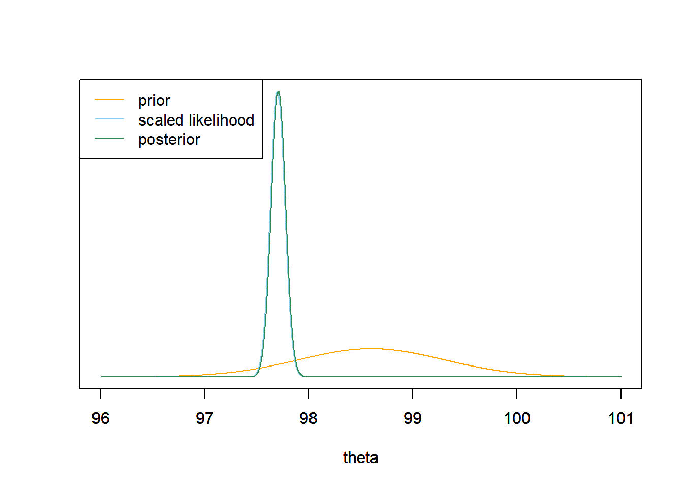
-
Since the posterior distribution is Normal, we can find the endpoints of the central 95% credible interval using the empirical rule: \(97.7 \pm 2 \times 0.07\). There is a posterior probability of 95% that population mean human body temperature is between 97.57 and 97.84 degrees Fahrenheit.
-
Remember that in JAGS
dnormis parametrized by the precision. The simulation results are consistent with the theory.Nrep = 10000 Nchains = 3 # data y = 97.7 n = 208 # model model_string <- "model{ # Likelihood y ~ dnorm(theta, n / sigma ^ 2) sigma <- 1 # Prior theta ~ dnorm(mu0, 1 / tau0 ^ 2) mu0 <- 98.6 tau0 <- 0.7 }" # Compile the model dataList = list(y=y, n=n) model <- jags.model(textConnection(model_string), data=dataList, n.chains=Nchains)## Compiling model graph ## Resolving undeclared variables ## Allocating nodes ## Graph information: ## Observed stochastic nodes: 1 ## Unobserved stochastic nodes: 1 ## Total graph size: 11 ## ## Initializing modelupdate(model, 1000, progress.bar= "none") posterior_sample <- coda.samples(model, variable.names= c("theta"), n.iter=Nrep, progress.bar= "none") # Summarize and check diagnostics summary(posterior_sample)## ## Iterations = 1001:11000 ## Thinning interval = 1 ## Number of chains = 3 ## Sample size per chain = 10000 ## ## 1. Empirical mean and standard deviation for each variable, ## plus standard error of the mean: ## ## Mean SD Naive SE Time-series SE ## 97.7088497 0.0693596 0.0004004 0.0004005 ## ## 2. Quantiles for each variable: ## ## 2.5% 25% 50% 75% 97.5% ## 97.57 97.66 97.71 97.76 97.85
-
Simulate a value of \(\theta\) from its posterior distribution, then given \(\theta\) simulate a value of \(Y\) from a Normal(\(\theta\), 1) distribution, and repeat many times.
theta_sim = rnorm(10000, mu_n, tau_n) y_sim = rnorm(10000, theta_sim, sigma) hist(y_sim, freq = FALSE, xlab = "Body temperature (degrees F)", main = "Posterior predictive distribution")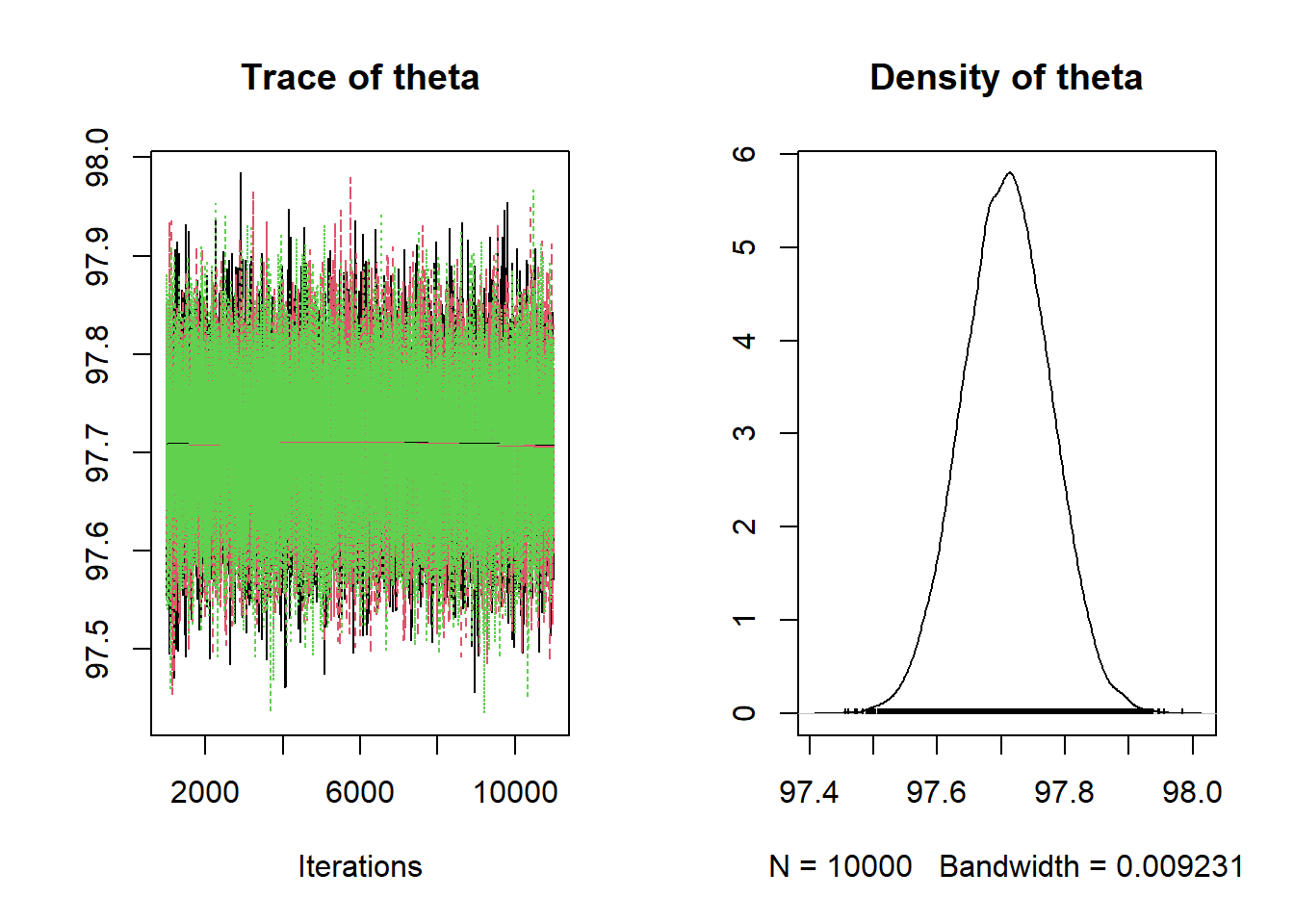
-
There is a posterior predictive probability of 95% that a randomly selected healthy human body temperature is between 95.7 and 99.7 degrees F. Very roughly, 95% of healthy human body temperatures are between 95.75 and 99.70 degrees F.
quantile(y_sim, c(0.025, 0.975))## 2.5% 97.5% ## 95.78790 99.70912
Example 11.3 Suppose that birthweights (grams) of human babies follow a Normal distribution with unknown mean \(\theta\) and known SD \(\sigma\). (1 pound \(\approx\) 454 grams.) Assume a Normal prior distribution for \(\theta\).
-
What do you think is a reasonable prior mean and prior SD?
-
Assume a prior mean of 3400 grams (about 7.5 pounds) and a prior SD of 225 grams (about 0.5 pounds). What do these assumptions say about \(\theta\)?
-
The following summarizes data on a random sample22 of 1000 live births in the U.S. in 2001.
data = read.csv("_data/birthweight.csv") y = data$birthweight hist(y, freq = FALSE, breaks = 50)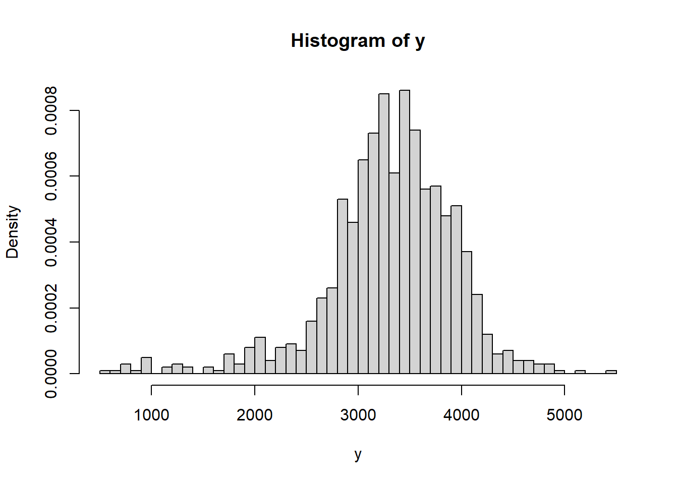
## Min. 1st Qu. Median Mean 3rd Qu. Max. ## 595 3005 3350 3315 3714 5500## [1] 631.3303n = length(y) ybar = mean(y) sigma = 600 # assumedDoes it seem reasonable to assume birthweights follow a Normal distribution?
-
Assume that \(\sigma = 600\) grams. Find the posterior distribution of \(\theta\) given the sample data.
-
Find and interpret a central 99% posterior credible interval for \(\theta\).
-
Use JAGS to approximate the posterior distribution. How do the results compare to the previous parts?
-
How could you use simulation (not JAGS) to approximate the posterior predictive distribution of birthweights?
-
Use the simulation from the previous part to find and interpret a 99% posterior prediction interval.
-
What percent of values in the sample fall outside the prediction interval? What does that tell you?
Solution. to Example 11.3
-
Depends on what you know about babies. But a prior mean in the 7-8 or so pounds range seems reasonable. The prior standard deviation represents your degree of uncertainty; what range of values do you think is plausible for mean birthweight?
-
We're pretty sure that mean birthweight is in the in the 7-8 pound range. Our prior probability that mean birthweight is between 3175 and 3625 grams (7-8 pounds) is about 68%. Our prior probability that mean birthweight is between 2950 and 3850 grams (6.5-8.5 pounds) is about 95%.
-
Assuming a Normal distribution doesn't seem terrible, but it does appear that maybe the tails are a little heavier than we would expect for a Normal distribution, especially at the low birthweights. That is, there might be some evidence in the data that extremely low (and maybe high) birthweights don't quite follow what would be expected if birthweights followed a Normal distribution.
-
With such a large sample size, the prior has very little influence and the posterior is almost entirely determined by the likelihood. The posterior mean is essentially the sample mean of 3315 grams (7.3 pounds). The posterior distribution is Normal with posterior mean 3315.6 grams and posterior SD 18.9 grams (about 0.04 pounds).
mu0 = 3400 tau0 = 225 tau_n = 1 / sqrt(n / sigma ^ 2 + 1 / tau0 ^ 2) mu_n = mu0 * (1 / tau0 ^ 2) / (1 / tau_n ^ 2) + ybar * (n / sigma ^ 2) / (1 / tau_n ^ 2)Prior Data (Sample Mean) Posterior Precision 0 0.0028 0.0028 SD 225 18.9737 18.9066 Mean 3400 3314.9590 3315.5595 theta = seq(mu0 - 3 * tau0, mu0 + 3 * tau0, 0.01) # the grid is just for plotting # prior prior = dnorm(theta, mu0, tau0) # likelihood likelihood = dnorm(ybar, theta, sigma / sqrt(n)) # posterior posterior = dnorm(theta, mu_n, tau_n) # plot ymax = max(c(prior, posterior)) scaled_likelihood = likelihood * ymax / max(likelihood) plot(theta, prior, type= 'l', col= 'orange', xlim= range(theta), ylim= c(0, ymax), ylab= '', yaxt= 'n') par(new=T) plot(theta, scaled_likelihood, type= 'l', col= 'skyblue', xlim= range(theta), ylim= c(0, ymax), ylab= '', yaxt= 'n') par(new=T) plot(theta, posterior, type= 'l', col= 'seagreen', xlim= range(theta), ylim= c(0, ymax), ylab= '', yaxt= 'n') legend("topleft", c("prior", "scaled likelihood", "posterior"), lty= 1, col= c("orange", "skyblue", "seagreen"))
-
The endpoints are \(3315.6\pm 2.6\times 18.9\).(The empirical rule multiplier for the middle 99% of values in a Normal distribution is about 2.6.) There is a posterior probability of 99% that population mean birthweight of babies23 in the U.S. is between 3266 and 3365 grams (about 7.2 to 7.4 pounds).
-
See the JAGS code a little further below. The results are similar to theory.
-
Simulate a value of \(\theta\) from its posterior distribution, then given \(\theta\) simulate a value of \(Y\) from a Normal(\(\theta\), \(\sigma = 600\)) distribution, and repeat many times.
theta_sim = rnorm(10000, mu_n, tau_n) y_sim = rnorm(10000, theta_sim, sigma) hist(y_sim, freq = FALSE, breaks = 50, xlab = "Birthweight (grams)", main = "Posterior predictive distribution")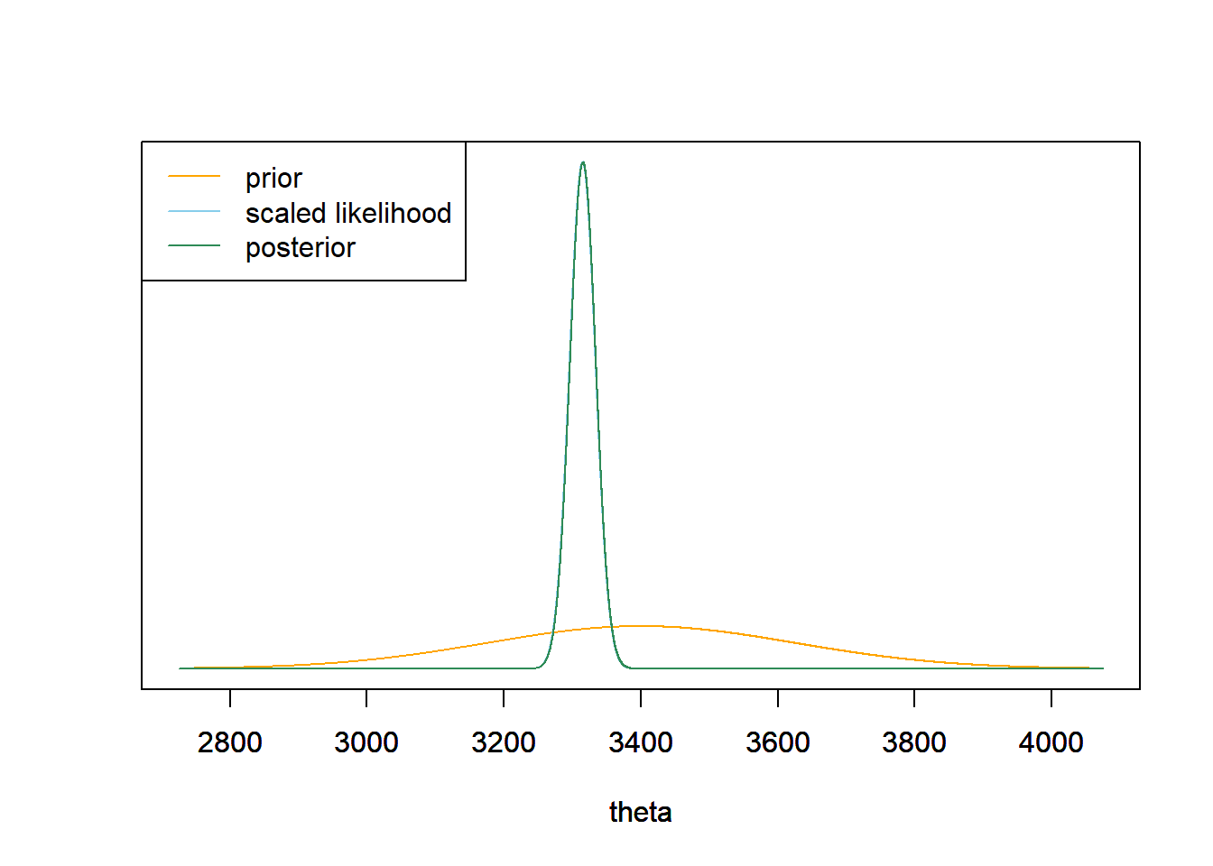
-
There is a posterior predictive probability of 99% that a randomly selected birthweight is between 1750 and 4830 grams. Very roughly, 99% of birthweights are between 1750 and 4830 grams.
quantile(y_sim, c(0.005, 0.995))## 0.5% 99.5% ## 1739.683 4820.684 -
About 3% of birthweights in the sample fall outside of the 99% prediction interval, when we would only expect 1%. While not a large difference in magnitude, we are obsering 3 times more values in the tails than we would expect if birthweights followed a Normal distribution. So we have some evidence that a Normal model might not be the best model for birthweights of all live births as it doesn't properly account for extreme birthweights. (Of course, it could be true that a Normal model is ok, but our assumed standard deviation of \(\sigma\) is wrong. But if we tried to increase \(\sigma\) to compensate for the extreme values, then the fit would get worse in the middle of the distribution.)
(sum(y < quantile(y_sim, 0.005)) + sum(y > quantile(y_sim, 0.995))) / n## [1] 0.029
In the temperature example, we were only provided the sample mean. In JAGS, we computed the likelihood of observing a sample of 97.7 in a sample of size 208 using dnorm(theta, n / sigma ^ 2). This likelihood represents a single observation of the sample mean in a sample of size 208.
In the birthweight example, we have the entire data set consisting of individual birthweights. While it is sufficient to know the sample mean to evaluate the likelihood, we can load the individual data values into JAGS. In fact, if we wanted to estimate the population standard deviation \(\sigma\) or other features of the population distribution, we would need to input all of the data; the sample mean alone would not be sufficient.
The JAGS code below takes the full sample of size 1000 as an input. Now the data consists of 1000 values each from a Normal(\(\theta\), \(\sigma\)) distribution. To find the likelihood of observing this sample, we evaluate the likelihood of each of the individual 1000 values in the data set, as in part 4 of Example 11.1. JAGS will then multiply these values together for us to find the likelihood of the sample. Notice how this is implemented in the code below. The vector y below represents the sample data consisting of 1000 values. The likelihood is now specified as a for loop which evaluates the likelihood y[i] ~ dnorm(theta, sigma) for each y[i] in the sample.
Nrep = 10000 Nchains = 3 # data # data has already been loaded in previous code # y is the full sample # n is the sample size # model model_string <- "model{ # Likelihood for (i in 1:n){ y[i] ~ dnorm(theta, 1 / sigma ^ 2) } sigma <- 600 # Prior theta ~ dnorm(mu0, 1 / tau0 ^ 2) mu0 <- 3400 tau0 <- 225 }" # Compile the model dataList = list(y=y, n=n) model <- jags.model(textConnection(model_string), data=dataList, n.chains=Nchains) ## Compiling model graph ## Resolving undeclared variables ## Allocating nodes ## Graph information: ## Observed stochastic nodes: 1000 ## Unobserved stochastic nodes: 1 ## Total graph size: 1011 ## ## Initializing model update(model, 1000, progress.bar= "none") posterior_sample <- coda.samples(model, variable.names= c("theta"), n.iter=Nrep, progress.bar= "none") # Summarize and check diagnostics summary(posterior_sample) ## ## Iterations = 1001:11000 ## Thinning interval = 1 ## Number of chains = 3 ## Sample size per chain = 10000 ## ## 1. Empirical mean and standard deviation for each variable, ## plus standard error of the mean: ## ## Mean SD Naive SE Time-series SE ## 3315.4132 18.7926 0.1085 0.1085 ## ## 2. Quantiles for each variable: ## ## 2.5% 25% 50% 75% 97.5% ## 3278 3303 3316 3328 3352 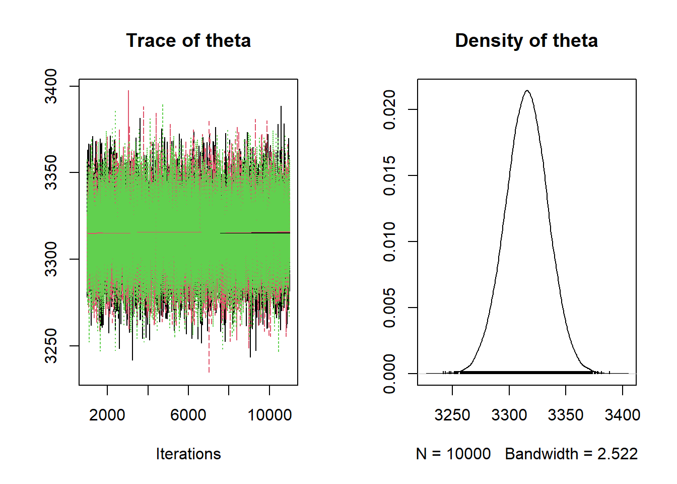
Example 11.4 Continuing the previous example. A Normal distribution model for birthweights doesn't appear to be the greatest fit for the data. There appears to be a higher percentage of extremely low birthweight babies than you would expect from a Normal distribution.
In this problem we will (1) use posterior predictive checking to assess the reasonableness of the assumption of Normality for birtweights, and (2) suggest an alternative model.
- How could you use posterior predictive simulation to simulate what a sample of 1000 birthweights might look like under this model. Simulate many such samples. Does the observed sample seem consistent with the model?
- Rather than comparing whole samples, we could compare the observed value of a summary statistic with what we would expect to see under the model. Suggest a statistic to use, then simulate the posterior predictive distribution of the statistic. Does the observed value of the statistic seem consistent with the model.
Solution. to Example 11.4
-
Simulate a value of \(\theta\) from its N(3315, 18.9) posterior distribution. Given \(\theta\), simulate 1000 values from a \(N(\theta, \sigma = 600)\) distribution, and plot those values to see what one sample might look like under this model. Repeat many times to generate many hypothetical samples and compare with the observed data. The plot shows the histogram of the observed data along with the density plot for each of 100 simulated samples of size 1000. Again, while not a terrible fit, there do seem to be more values in the tail (the lower tail especially) than would be expected under this model.
# plot the observed data hist(y, freq = FALSE, breaks = 50) # observed data # number of samples to simulate n_samples = 100 # simulate thetas from posterior theta = rnorm(n_samples, mu_n, tau_n) # simulate samples for (r in 1 :n_samples){ # simulate values from N(theta, sigma) distribution y_sim = rnorm(n, theta[r], sigma) # add plot of simulated sample to histogram lines(density(y_sim), col = rgb(135, 206, 235, max = 255, alpha = 25)) }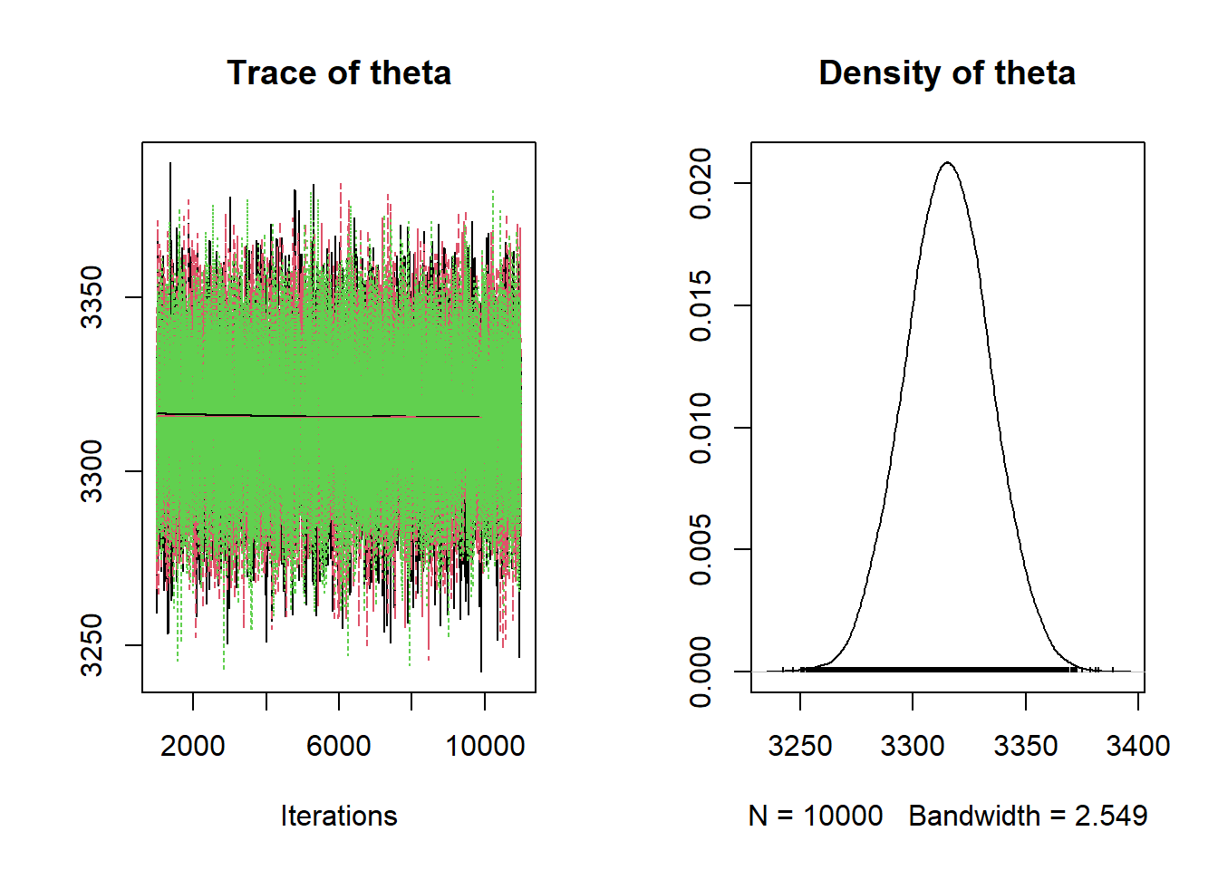
-
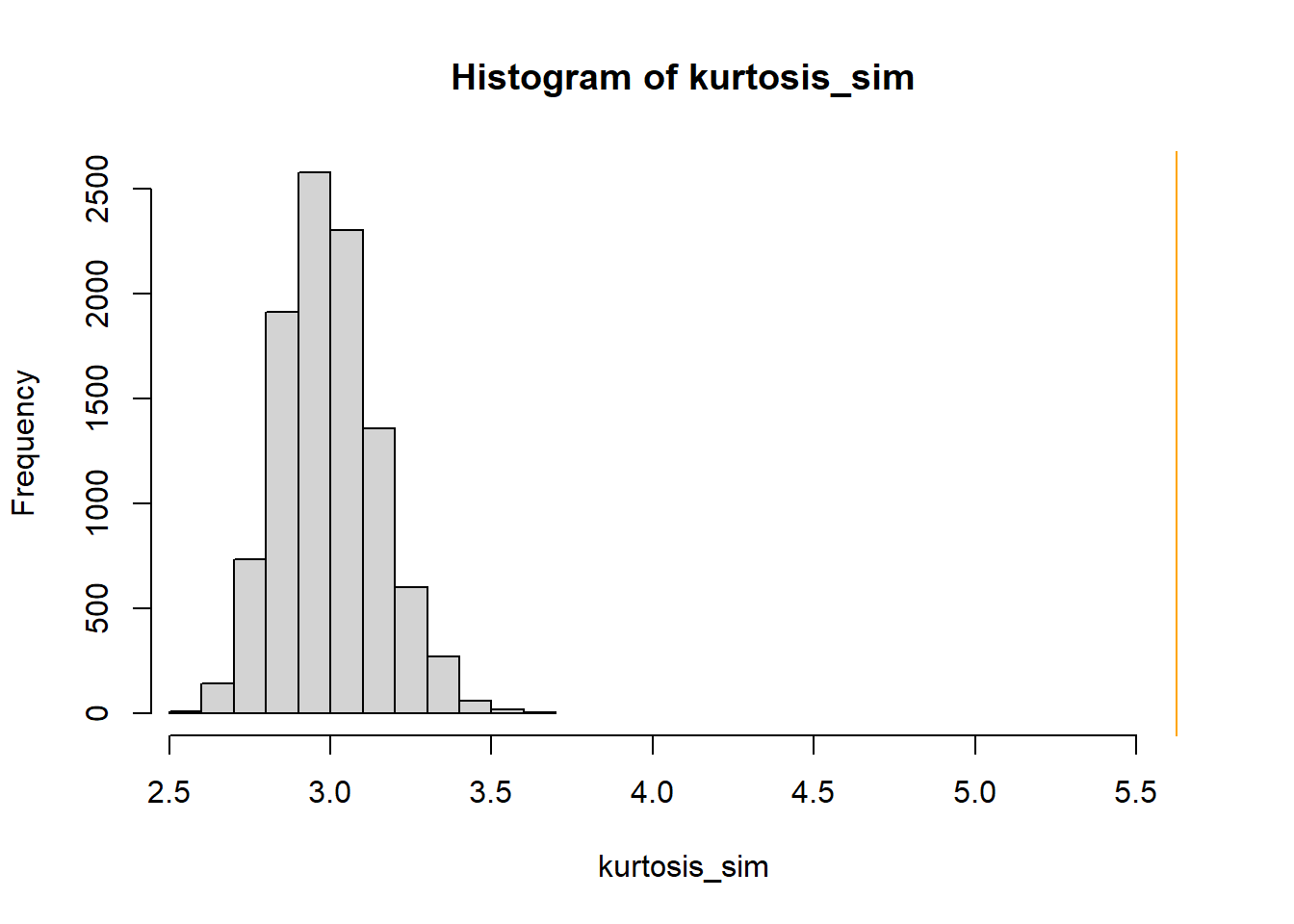
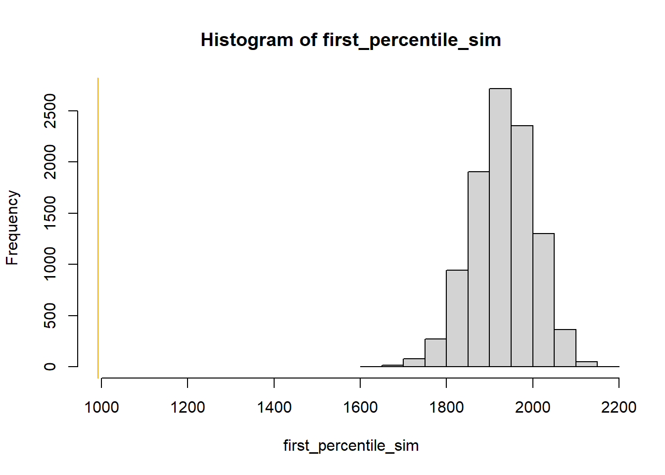
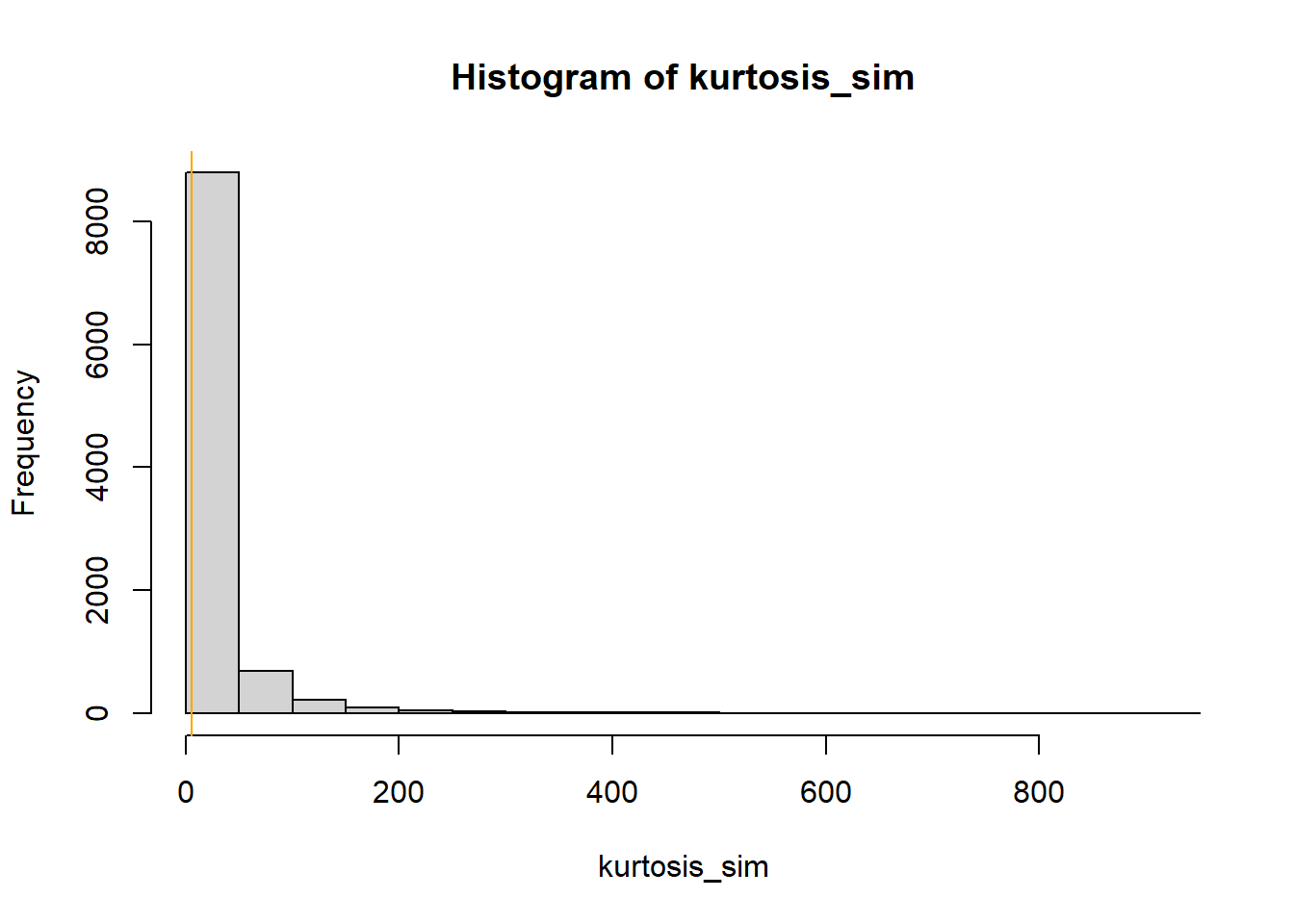
We could look at the minimum value in the sample, but this would be heavily influenced by just a single outlier. To see the whole tail a little better, we could look at a small percentile, say the first percentile. There are many other choices. In particular, the kurtosis 24 statistic is a measure of how heavy the tails are. Whatever statistic we choose, we conduct the simulation similar to the previous part. Simulate a value of \(\theta\) from its N(3315, 18.9) posterior distribution. Given \(\theta\), simulate 1000 values from a \(N(\theta, \sigma = 600)\) distribution, and compute the statistic (first percentile, kurtosis). Repeat many times to see what values of the statistic would be expected under the model. Then compare the observed statistic against the simulated values. For either statistic, the observed value is way more extreme than we would expect under a Normal model. So it appears that a Normal likelihood does not full describe the distribution of birthweights for all live births.
library(moments) # number of samples to simulate n_samples = 10000 # simulate thetas from posterior theta = rnorm(n_samples, mu_n, tau_n) # to store "test" statistic first_percentile_sim = rep(NA, n_samples) kurtosis_sim = rep(NA, n_samples) # simulate samples for (r in 1 :n_samples){ # simulate values from N(theta, sigma) distribution y_sim = rnorm(n, theta[r], sigma) # compute "test" statistic for simulated sample first_percentile_sim[r] = quantile(y_sim, 0.01) kurtosis_sim[r] = kurtosis(y_sim) } # plot and compare observed value first_percentile_obs = quantile(y, 0.01) hist(first_percentile_sim, xlim = range(c(first_percentile_obs, first_percentile_sim))) abline(v = first_percentile_obs, col = "orange") kurtosis_obs = kurtosis(y) hist(kurtosis_sim, xlim = range(c(kurtosis_obs, kurtosis_sim))) abline(v = kurtosis_obs, col = "orange")
The Normal-Normal model assumes that the population distribution of individual values of the measured numerical variable is Normal — that is, a Normal likelihood. Posterior predictive checking can be used to assess whether a Normal likelihood is appropriate for the observed data. If a Normal likelihood isn't an appropriate model for the data then other likelihood functions can be used. In particular, if the observed data is relatively unimodal and symmetric but has more extreme values than can be accommodated by a Normal likelihood, a \(t\)-distribution or other distribution with heavy tails can be used to model the likelihood.
If the observed data seems to be skewed or have multiple modes, then maybe other parameters (median, mode) are more appropriate measures of center than the population mean
Normal distributions don't allow much room for extreme values. An alternative is to assume a distribution with heavier tails. For example, t-distributions have heavier tails than Normal. For t-distributions, the degrees of freedom parameter control how heavy the tails are.
Using a likelihood based on a t-distribution centered at \(\theta\) with a Normal distribution prior for \(\theta\) does not lead to a recognizable posterior. So we'll use JAGS to approximate the posterior distribution. We'll assume 3 degrees of freedom for illustration. However, in practice the degrees of freedom is another parameter that would be estimated from data, just like \(\sigma\). Note the dt in the likelihood which has the additional degrees of freedom parameter. (For a t-distribution with \(d\) degrees of freedom the variance is \(d/(d-2)\) for \(d>2\), and the JAGS parametrization is based on this.)
Nrep = 10000 Nchains = 3 # data # data has already been loaded in previous code # y is the full sample # n is the sample size # model model_string <- "model{ # Likelihood for (i in 1:n){ y[i] ~ dt(theta, (1 / sigma ^ 2) / (tdf / (tdf - 2)), tdf) } sigma <- 600 tdf <- 3 # Prior theta ~ dnorm(mu0, 1 / tau0 ^ 2) mu0 <- 3400 tau0 <- 225 }" # Compile the model dataList = list(y=y, n=n) model <- jags.model(textConnection(model_string), data=dataList, n.chains=Nchains) ## Compiling model graph ## Resolving undeclared variables ## Allocating nodes ## Graph information: ## Observed stochastic nodes: 1000 ## Unobserved stochastic nodes: 1 ## Total graph size: 1015 ## ## Initializing model update(model, 1000, progress.bar= "none") posterior_sample <- coda.samples(model, variable.names= c("theta"), n.iter=Nrep, progress.bar= "none") # Summarize and check diagnostics summary(posterior_sample) ## ## Iterations = 2001:12000 ## Thinning interval = 1 ## Number of chains = 3 ## Sample size per chain = 10000 ## ## 1. Empirical mean and standard deviation for each variable, ## plus standard error of the mean: ## ## Mean SD Naive SE Time-series SE ## 3348.0463 31.6359 0.1826 0.2286 ## ## 2. Quantiles for each variable: ## ## 2.5% 25% 50% 75% 97.5% ## 3286 3327 3348 3369 3411 
The posterior distribution of \(\theta\) is similar to the one from the Normal likelihood model, but it does change a little bit.
We'll now try posterior predictive checks. We use the simulated values of \(\theta\) from JAGS. For each value of \(\theta\), we generate a sample of size 1000 from a t-distribution centered at \(\theta\) and with a standard deviation of 600. (rt in R returns values on a standardized scale which we then rescale.)
tdf = 3 sigma = 600 / sqrt(tdf / (tdf - 2)) # plot the observed data hist(y, freq = FALSE, breaks = 50) # observed data # number of samples to simulate n_samples = 100 # simulate thetas from posterior theta = as.matrix(posterior_sample) # simulate samples for (r in 1 :n_samples){ # simulate values from a t-distribution y_sim = theta[r] + sigma * rt(n, tdf) # add plot of simulated sample to histogram lines(density(y_sim), col = rgb(135, 206, 235, max = 255, alpha = 25)) } 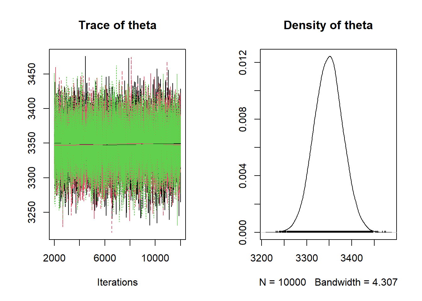
We see that the actual sample resembles simulated samples more closely for the model based on the t-distribution likelihood than for the one based on the Normal likelihood. We can also consider summary statistics measuring the "tailed-ness" as before.
# number of samples to simulate n_samples = 10000 # to store "test" statistic first_percentile_sim = rep(NA, n_samples) kurtosis_sim = rep(NA, n_samples) # simulate samples for (r in 1 :n_samples){ # simulate values from a t-distribution y_sim = theta[r] + sigma * rt(n, tdf) # compute "test" statistic for simulated sample first_percentile_sim[r] = quantile(y_sim, 0.01) kurtosis_sim[r] = kurtosis(y_sim) } # plot and compare observed value first_percentile_obs = quantile(y, 0.01) hist(first_percentile_sim, xlim = range(c(first_percentile_obs, first_percentile_sim))) abline(v = first_percentile_obs, col = "orange") kurtosis_obs = kurtosis(y) hist(kurtosis_sim, xlim = range(c(kurtosis_obs, kurtosis_sim))) abline(v = kurtosis_obs, col = "orange") 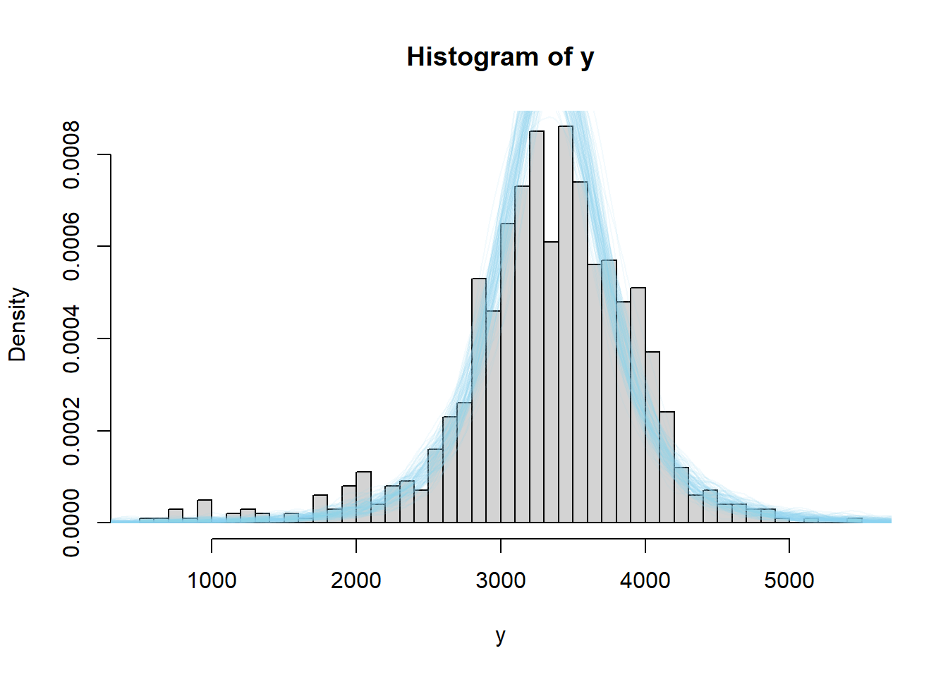
The observed sample kurtosis is in line with what we would expect under the model. The observed first percentile is still extreme relative to what we would expect from the model, but not as extreme as it was under the Normal model.
While we do want a model that fits the data well, we also do not want to risk overfitting the data. In this case, we do not want a few extreme outliers to unduly influence the model. However, it does appear that a model that allows for heavier tails than a Normal distribution could be useful here.
How to Find Population Mean From Sample Using Bayesian Methods
Source: https://bookdown.org/kevin_davisross/bayesian-reasoning-and-methods/mean.html